데이콘 Basic 여행상품 신청예측
from google.colab import drive
drive.mount('/content/drive')
Mounted at /content/drive
0.준비
import pandas as pd
train = pd.read_csv('/content/drive/MyDrive/data/여행상품신청/train.csv')
test = pd.read_csv('/content/drive/MyDrive/data/여행상품신청/test.csv')
sample_submission = pd.read_csv('/content/drive/MyDrive/data/여행상품신청/sample_submission.csv')
- id : 샘플 아이디
- Age : 나이
- TypeofContact : 고객의 제품 인지 방법 (회사의 홍보 or 스스로 검색)
- CityTier : 주거 중인 도시의 등급. (인구, 시설, 생활 수준 기준) (1등급 > 2등급 > 3등급)
- DurationOfPitch : 영업 사원이 고객에게 제공하는 프레젠테이션 기간
- Occupation : 직업
- Gender : 성별
- NumberOfPersonVisiting : 고객과 함께 여행을 계획 중인 총 인원
- NumberOfFollowups : 영업 사원의 프레젠테이션 후 이루어진 후속 조치 수
- ProductPitched : 영업 사원이 제시한 상품
- PreferredPropertyStar : 선호 호텔 숙박업소 등급
- MaritalStatus : 결혼여부
- NumberOfTrips : 평균 연간 여행 횟수
- Passport : 여권 보유 여부 (0: 없음, 1: 있음)
- PitchSatisfactionScore : 영업 사원의 프레젠테이션 만족도
- OwnCar : 자동차 보유 여부 (0: 없음, 1: 있음)
- NumberOfChildrenVisiting : 함께 여행을 계획 중인 5세 미만의 어린이 수
- Designation : (직업의) 직급
- MonthlyIncome : 월 급여
- ProdTaken : 여행 패키지 신청 여부 (0: 신청 안 함, 1: 신청함)
train
| id | Age | TypeofContact | CityTier | DurationOfPitch | Occupation | Gender | NumberOfPersonVisiting | NumberOfFollowups | ProductPitched | PreferredPropertyStar | MaritalStatus | NumberOfTrips | Passport | PitchSatisfactionScore | OwnCar | NumberOfChildrenVisiting | Designation | MonthlyIncome | ProdTaken | |
|---|---|---|---|---|---|---|---|---|---|---|---|---|---|---|---|---|---|---|---|---|
| 0 | 1 | 28.0 | Company Invited | 1 | 10.0 | Small Business | Male | 3 | 4.0 | Basic | 3.0 | Married | 3.0 | 0 | 1 | 0 | 1.0 | Executive | 20384.0 | 0 |
| 1 | 2 | 34.0 | Self Enquiry | 3 | NaN | Small Business | Female | 2 | 4.0 | Deluxe | 4.0 | Single | 1.0 | 1 | 5 | 1 | 0.0 | Manager | 19599.0 | 1 |
| 2 | 3 | 45.0 | Company Invited | 1 | NaN | Salaried | Male | 2 | 3.0 | Deluxe | 4.0 | Married | 2.0 | 0 | 4 | 1 | 0.0 | Manager | NaN | 0 |
| 3 | 4 | 29.0 | Company Invited | 1 | 7.0 | Small Business | Male | 3 | 5.0 | Basic | 4.0 | Married | 3.0 | 0 | 4 | 0 | 1.0 | Executive | 21274.0 | 1 |
| 4 | 5 | 42.0 | Self Enquiry | 3 | 6.0 | Salaried | Male | 2 | 3.0 | Deluxe | 3.0 | Divorced | 2.0 | 0 | 3 | 1 | 0.0 | Manager | 19907.0 | 0 |
| ... | ... | ... | ... | ... | ... | ... | ... | ... | ... | ... | ... | ... | ... | ... | ... | ... | ... | ... | ... | ... |
| 1950 | 1951 | 28.0 | Self Enquiry | 1 | 10.0 | Small Business | Male | 3 | 5.0 | Basic | 3.0 | Single | 2.0 | 0 | 1 | 1 | 2.0 | Executive | 20723.0 | 0 |
| 1951 | 1952 | 41.0 | Self Enquiry | 3 | 8.0 | Salaried | Female | 3 | 3.0 | Super Deluxe | 5.0 | Divorced | 1.0 | 0 | 5 | 1 | 1.0 | AVP | 31595.0 | 0 |
| 1952 | 1953 | 38.0 | Company Invited | 3 | 28.0 | Small Business | Female | 3 | 4.0 | Basic | 3.0 | Divorced | 7.0 | 0 | 2 | 1 | 2.0 | Executive | 21651.0 | 0 |
| 1953 | 1954 | 28.0 | Self Enquiry | 3 | 30.0 | Small Business | Female | 3 | 5.0 | Deluxe | 3.0 | Married | 3.0 | 0 | 1 | 1 | 2.0 | Manager | 22218.0 | 0 |
| 1954 | 1955 | 22.0 | Company Invited | 1 | 9.0 | Salaried | Male | 2 | 4.0 | Basic | 3.0 | Divorced | 1.0 | 1 | 3 | 0 | 0.0 | Executive | 17853.0 | 1 |
1955 rows × 20 columns
0.1.데이터 전처리
0.1.1.결측치 처리
train.isna().sum()
id                            0
Age                          94
TypeofContact                10
CityTier                      0
DurationOfPitch             102
Occupation                    0
Gender                        0
NumberOfPersonVisiting        0
NumberOfFollowups            13
ProductPitched                0
PreferredPropertyStar        10
MaritalStatus                 0
NumberOfTrips                57
Passport                      0
PitchSatisfactionScore        0
OwnCar                        0
NumberOfChildrenVisiting     27
Designation                   0
MonthlyIncome               100
ProdTaken                     0
dtype: int64
test.isna().sum()
id                            0
Age                         132
TypeofContact                15
CityTier                      0
DurationOfPitch             149
Occupation                    0
Gender                        0
NumberOfPersonVisiting        0
NumberOfFollowups            32
ProductPitched                0
PreferredPropertyStar        16
MaritalStatus                 0
NumberOfTrips                83
Passport                      0
PitchSatisfactionScore        0
OwnCar                        0
NumberOfChildrenVisiting     39
Designation                   0
MonthlyIncome               133
dtype: int64
def handle_na(data):
    temp = data.copy()
    for col, dtype in temp.dtypes.items():
        if dtype == 'object':
            # 문자형 칼럼의 경우 'Unknown'을 채워줍니다.
            value = 'Unknown'
        elif dtype == int or dtype == float:
            # 수치형 칼럼의 경우 0을 채워줍니다.
            value = 0
        temp.loc[:,col] = temp[col].fillna(value)
    return temp

train_nona = handle_na(train)

# 결측치 처리가 잘 되었는지 확인해 줍니다.
train_nona.isna().sum()
id                          0
Age                         0
TypeofContact               0
CityTier                    0
DurationOfPitch             0
Occupation                  0
Gender                      0
NumberOfPersonVisiting      0
NumberOfFollowups           0
ProductPitched              0
PreferredPropertyStar       0
MaritalStatus               0
NumberOfTrips               0
Passport                    0
PitchSatisfactionScore      0
OwnCar                      0
NumberOfChildrenVisiting    0
Designation                 0
MonthlyIncome               0
ProdTaken                   0
dtype: int64
0.1.2.문자형 변수 전처리
object_columns = train_nona.columns[train_nona.dtypes == 'object']
print('object 칼럼은 다음과 같습니다 : ', list(object_columns))

# 해당 칼럼만 보아서 봅시다
train_nona[object_columns]
object 칼럼은 다음과 같습니다 : ['TypeofContact', 'Occupation', 'Gender', 'ProductPitched', 'MaritalStatus', 'Designation']
| TypeofContact | Occupation | Gender | ProductPitched | MaritalStatus | Designation | |
|---|---|---|---|---|---|---|
| 0 | Company Invited | Small Business | Male | Basic | Married | Executive |
| 1 | Self Enquiry | Small Business | Female | Deluxe | Single | Manager |
| 2 | Company Invited | Salaried | Male | Deluxe | Married | Manager |
| 3 | Company Invited | Small Business | Male | Basic | Married | Executive |
| 4 | Self Enquiry | Salaried | Male | Deluxe | Divorced | Manager |
| ... | ... | ... | ... | ... | ... | ... |
| 1950 | Self Enquiry | Small Business | Male | Basic | Single | Executive |
| 1951 | Self Enquiry | Salaried | Female | Super Deluxe | Divorced | AVP |
| 1952 | Company Invited | Small Business | Female | Basic | Divorced | Executive |
| 1953 | Self Enquiry | Small Business | Female | Deluxe | Married | Manager |
| 1954 | Company Invited | Salaried | Male | Basic | Divorced | Executive |
1955 rows × 6 columns
train_nona['Gender'].value_counts()
Male       1207
Female      692
Fe Male      56
Name: Gender, dtype: int64
train_nona.loc[train_nona['Gender']=='Fe Male','Gender'] = 'Female'
test.loc[test['Gender']=='Fe Male','Gender'] = 'Female'
train_nona['Gender'].value_counts()
Male      1207
Female     748
Name: Gender, dtype: int64
# LabelEncoder를 준비해줍니다.
from sklearn.preprocessing import LabelEncoder

encoder = LabelEncoder()

# LabelEcoder는 학습하는 과정을 필요로 합니다.
encoder.fit(train_nona['TypeofContact'])

#학습된 encoder를 사용하여 문자형 변수를 숫자로 변환해줍니다.
encoder.transform(train_nona['TypeofContact'])
array([0, 1, 0, ..., 0, 1, 0])
train_enc = train_nona.copy()

# 모든 문자형 변수에 대해 encoder를 적용합니다.
for o_col in object_columns:
    encoder = LabelEncoder()
    encoder.fit(train_enc[o_col])
    train_enc[o_col] = encoder.transform(train_enc[o_col])

# 결과를 확인합니다.
train_enc
| id | Age | TypeofContact | CityTier | DurationOfPitch | Occupation | Gender | NumberOfPersonVisiting | NumberOfFollowups | ProductPitched | PreferredPropertyStar | MaritalStatus | NumberOfTrips | Passport | PitchSatisfactionScore | OwnCar | NumberOfChildrenVisiting | Designation | MonthlyIncome | ProdTaken | |
|---|---|---|---|---|---|---|---|---|---|---|---|---|---|---|---|---|---|---|---|---|
| 0 | 1 | 28.0 | 0 | 1 | 10.0 | 3 | 1 | 3 | 4.0 | 0 | 3.0 | 1 | 3.0 | 0 | 1 | 0 | 1.0 | 1 | 20384.0 | 0 |
| 1 | 2 | 34.0 | 1 | 3 | 0.0 | 3 | 0 | 2 | 4.0 | 1 | 4.0 | 2 | 1.0 | 1 | 5 | 1 | 0.0 | 2 | 19599.0 | 1 |
| 2 | 3 | 45.0 | 0 | 1 | 0.0 | 2 | 1 | 2 | 3.0 | 1 | 4.0 | 1 | 2.0 | 0 | 4 | 1 | 0.0 | 2 | 0.0 | 0 |
| 3 | 4 | 29.0 | 0 | 1 | 7.0 | 3 | 1 | 3 | 5.0 | 0 | 4.0 | 1 | 3.0 | 0 | 4 | 0 | 1.0 | 1 | 21274.0 | 1 |
| 4 | 5 | 42.0 | 1 | 3 | 6.0 | 2 | 1 | 2 | 3.0 | 1 | 3.0 | 0 | 2.0 | 0 | 3 | 1 | 0.0 | 2 | 19907.0 | 0 |
| ... | ... | ... | ... | ... | ... | ... | ... | ... | ... | ... | ... | ... | ... | ... | ... | ... | ... | ... | ... | ... |
| 1950 | 1951 | 28.0 | 1 | 1 | 10.0 | 3 | 1 | 3 | 5.0 | 0 | 3.0 | 2 | 2.0 | 0 | 1 | 1 | 2.0 | 1 | 20723.0 | 0 |
| 1951 | 1952 | 41.0 | 1 | 3 | 8.0 | 2 | 0 | 3 | 3.0 | 4 | 5.0 | 0 | 1.0 | 0 | 5 | 1 | 1.0 | 0 | 31595.0 | 0 |
| 1952 | 1953 | 38.0 | 0 | 3 | 28.0 | 3 | 0 | 3 | 4.0 | 0 | 3.0 | 0 | 7.0 | 0 | 2 | 1 | 2.0 | 1 | 21651.0 | 0 |
| 1953 | 1954 | 28.0 | 1 | 3 | 30.0 | 3 | 0 | 3 | 5.0 | 1 | 3.0 | 1 | 3.0 | 0 | 1 | 1 | 2.0 | 2 | 22218.0 | 0 |
| 1954 | 1955 | 22.0 | 0 | 1 | 9.0 | 2 | 1 | 2 | 4.0 | 0 | 3.0 | 0 | 1.0 | 1 | 3 | 0 | 0.0 | 1 | 17853.0 | 1 |
1955 rows × 20 columns
# 결측치 처리
test = handle_na(test)

# 문자형 변수 전처리
for o_col in object_columns:
    encoder = LabelEncoder()

    # test 데이터를 이용해 encoder를 학습하는 것은 Data Leakage 입니다! 조심!
    encoder.fit(train_nona[o_col])

    # test 데이터는 오로지 transform 에서만 사용되어야 합니다.
    test[o_col] = encoder.transform(test[o_col])

# 결과를 확인합니다.
test
| id | Age | TypeofContact | CityTier | DurationOfPitch | Occupation | Gender | NumberOfPersonVisiting | NumberOfFollowups | ProductPitched | PreferredPropertyStar | MaritalStatus | NumberOfTrips | Passport | PitchSatisfactionScore | OwnCar | NumberOfChildrenVisiting | Designation | MonthlyIncome | |
|---|---|---|---|---|---|---|---|---|---|---|---|---|---|---|---|---|---|---|---|
| 0 | 1 | 0.524590 | 0 | 3 | 0.000000 | 3 | 1 | 2 | 5.0 | 1 | 3.0 | 1 | 1.0 | 0 | 2 | 0 | 1.0 | 2 | -0.363121 |
| 1 | 2 | 0.754098 | 1 | 2 | 0.305556 | 3 | 1 | 3 | 0.0 | 1 | 4.0 | 1 | 1.0 | 1 | 5 | 0 | 1.0 | 2 | -0.316471 |
| 2 | 3 | 0.606557 | 1 | 3 | 0.611111 | 3 | 1 | 3 | 4.0 | 1 | 3.0 | 1 | 5.0 | 0 | 5 | 1 | 0.0 | 2 | -0.142953 |
| 3 | 4 | 0.704918 | 1 | 1 | 1.000000 | 3 | 1 | 3 | 6.0 | 1 | 3.0 | 3 | 6.0 | 0 | 3 | 1 | 2.0 | 2 | 0.070608 |
| 4 | 5 | 0.409836 | 1 | 3 | 0.194444 | 1 | 0 | 4 | 4.0 | 0 | 4.0 | 3 | 3.0 | 1 | 4 | 1 | 3.0 | 1 | -0.070797 |
| ... | ... | ... | ... | ... | ... | ... | ... | ... | ... | ... | ... | ... | ... | ... | ... | ... | ... | ... | ... |
| 2928 | 2929 | 0.885246 | 1 | 1 | 0.166667 | 3 | 0 | 2 | 3.0 | 4 | 3.0 | 2 | 7.0 | 0 | 4 | 1 | 1.0 | 0 | 1.309948 |
| 2929 | 2930 | 0.540984 | 1 | 1 | 0.250000 | 3 | 0 | 4 | 2.0 | 1 | 3.0 | 3 | 2.0 | 0 | 3 | 0 | 1.0 | 2 | 0.174085 |
| 2930 | 2931 | 0.540984 | 0 | 1 | 0.861111 | 2 | 1 | 4 | 4.0 | 1 | 3.0 | 0 | 3.0 | 0 | 4 | 1 | 1.0 | 2 | 0.207652 |
| 2931 | 2932 | 0.426230 | 1 | 1 | 0.250000 | 3 | 1 | 4 | 2.0 | 0 | 5.0 | 3 | 2.0 | 0 | 2 | 1 | 3.0 | 1 | -0.041459 |
| 2932 | 2933 | 0.508197 | 1 | 1 | 0.250000 | 2 | 1 | 3 | 5.0 | 1 | 3.0 | 0 | 3.0 | 0 | 4 | 1 | 1.0 | 2 | 0.054749 |
2933 rows × 19 columns
0.1.3.(추가) 결측치 처리 모듈 생성
- 0으로 채운 수치형 컬럼의 결측치를 회귀예측 모델로 예측하여 채워넣는 모듈 생성
from sklearn.ensemble import RandomForestRegressor
from sklearn.model_selection import train_test_split
from sklearn.metrics import mean_absolute_error
from sklearn.ensemble import ExtraTreesRegressor
def prod_val(feature:str):
  if len(train_enc[train_enc[feature]==0])==0:
    return 'already processed'
  train_temp = train_enc[train_enc[feature]!=0]

  features = train_temp.columns[1:-1].drop(feature)
  target = feature

  X = train_temp[features]
  y = train_temp[target]

  X_train,X_test,y_train,y_test = train_test_split(X,y,train_size=0.9,shuffle=False)
  model_rf = ExtraTreesRegressor(n_estimators=300)

  model_rf.fit(X_train,y_train)

  train_predict = model_rf.predict(X_test)

  print(f'{feature} MAE: {mean_absolute_error(train_predict,y_test)}')

  X = train_enc[train_enc[feature]==0][features]

  train_enc.loc[train_enc[feature]==0,feature] = model_rf.predict(X)

  test_temp = test[test[feature]==0]

  X = test_temp[features]

  test.loc[test[feature]==0,feature] = model_rf.predict(X)

  print(f'\ntrain set: \n{train_enc[feature].value_counts().sort_index().head(3)}')
  print(f'\ntest set: \n{test[feature].value_counts().sort_index().head(3)}')
1.EDA
import seaborn as sns
import matplotlib.pyplot as plt
import numpy as np
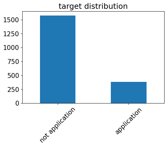
1.1.target
plt.figure(dpi=100)
train_enc['ProdTaken'].value_counts().plot(kind='bar')
plt.title('target distribution')
plt.xticks(np.arange(2),labels = ['not application','application'],rotation=45)
plt.show()
1.2.feature & target
1.2.1.Feature correlatoin(feature importances)
y = np.arange(len(train_enc.corr()['ProdTaken'].values))
ind = train_enc.corr()['ProdTaken'].index

values = abs(train_enc.corr()['ProdTaken'].values)

plt.figure(dpi=150)

plt.title('Feature correlation with target')
plt.barh(y,values)
plt.yticks(y,ind)

plt.show()
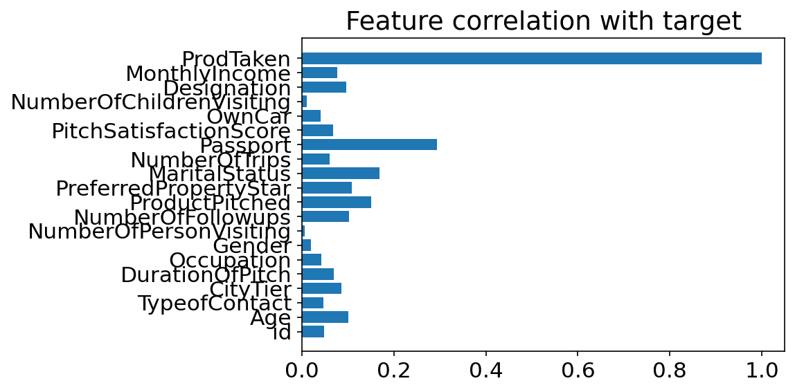
- 여권의 유무가 target과 가장 상관관계가 높은 것을 알 수 있다.
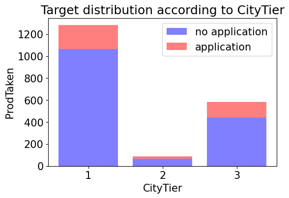
1.2.2.CityTier ~ target
train_enc.groupby(['CityTier','ProdTaken'])['id'].count()
CityTier  ProdTaken
1         0            1065
          1             218
2         0              66
          1              24
3         0             441
          1             141
Name: id, dtype: int64
temp = train_enc.groupby(['CityTier','ProdTaken'])['id'].count().values
temp
array([1065, 218, 66, 24, 441, 141])
no_application = temp[[0,2,4]]
application = temp[[1,3,5]]
alpha = 0.5
no_application
array([1065, 66, 441])
plt.figure(dpi=100)
p1 = plt.bar(np.arange(3), no_application, color='b', alpha=alpha)
p2 = plt.bar(np.arange(3), application, color='r', alpha=alpha,bottom=no_application) # stacked bar chart

plt.title('Target distribution according to CityTier')
plt.xlabel('CityTier')
plt.ylabel('ProdTaken')
plt.xticks(np.arange(3),labels=[1,2,3])
plt.legend((p1[0],p2[0]),('no application','application'))
plt.show()
ratio  = application / no_application
plt.figure(dpi=100)
plt.bar(np.arange(3),ratio)
plt.xlabel('CityTier')
plt.title('application ratio')
plt.xticks(np.arange(3),labels=[1,2,3])
plt.show()
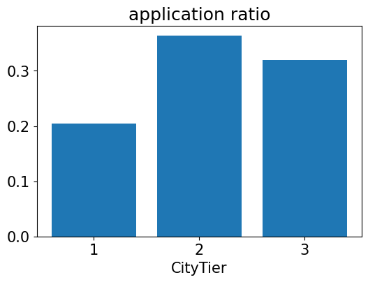
- 그래프를 통해 2등급 도시에는 주거 중인 시민이 별로 없다는 것을 알 수 있다.
- 또한 신청자 수는 1등급 도시에서 가장 많았지만 각 도시별 신청자 수 비율을 보면 2등급 도시가 가장 높은 것을 알 수 있다.
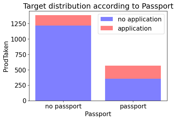
1.2.3.Passport ~ target
train_enc.groupby(['Passport','ProdTaken'])['id'].count()
Passport  ProdTaken
0         0            1218
          1             168
1         0             354
          1             215
Name: id, dtype: int64
temp = train_enc.groupby(['Passport','ProdTaken'])['id'].count().values
temp
array([1218, 168, 354, 215])
no_application = temp[[0,2]]
application = temp[[1,3]]
alpha = 0.5
no_application
array([1218, 354])
plt.figure(dpi=100)
p1 = plt.bar(np.arange(2), no_application, color='b', alpha=alpha)
p2 = plt.bar(np.arange(2), application, color='r', alpha=alpha,bottom=no_application) # stacked bar chart

plt.title('Target distribution according to Passport')
plt.xlabel('Passport')
plt.ylabel('ProdTaken')
plt.xticks(np.arange(2),labels=['no passport','passport'])
plt.legend((p1[0],p2[0]),('no application','application'))
plt.show()
fig=plt.figure(figsize=(10,10), dpi=100)
(ax1, ax2)=fig.subplots(1,2).flatten()

temp = train_enc[train_enc['Passport']==0].reset_index(drop = True)
x = temp['ProdTaken'].value_counts()
x.plot.pie(ax=ax1)
_=ax1.set_title('no passport')
ax1.legend(bbox_to_anchor=(0.9, 1), loc=2,labels=['no application','application'])

temp = train_enc[train_enc['Passport']==1].reset_index(drop = True)
x = temp['ProdTaken'].value_counts()
x.plot.pie(ax=ax2)
_=ax2.set_title('have passport')


plt.show()
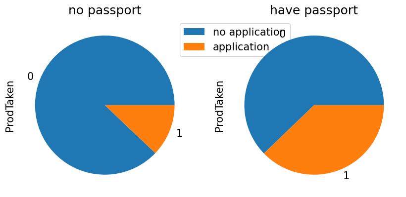
- 그래프를 통해 여권을 가지고 있는 사람은 가지고 있지 않는 사람보다 더 높은 비율로 신청을 하는 것으로 보인다. (어찌보면 당연한 결과이다.)
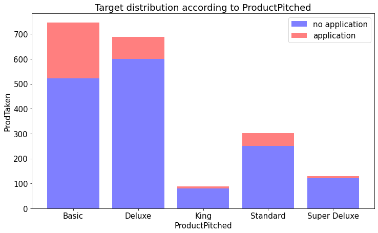
1.2.4. ProductPitched ~ target
train_nona['ProductPitched'].unique()
array(['Basic', 'Deluxe', 'King', 'Standard', 'Super Deluxe'],
      dtype=object)
train_nona.groupby(['ProductPitched','ProdTaken'])['id'].count()
ProductPitched  ProdTaken
Basic           0            522
                1            223
Deluxe          0            599
                1             90
King            0             80
                1              9
Standard        0            251
                1             51
Super Deluxe    0            120
                1             10
Name: id, dtype: int64
temp = train_nona.groupby(['ProductPitched','ProdTaken'])['id'].count().values
temp
array([522, 223, 599, 90, 80, 9, 251, 51, 120, 10])
ind = train_nona['ProductPitched'].unique()
ind
array(['Basic', 'Deluxe', 'King', 'Standard', 'Super Deluxe'],
      dtype=object)
no_application = temp[[0,2,4,6,8]]
application = temp[[1,3,5,7,9]]
alpha = 0.5
no_application
array([522, 599, 80, 251, 120])
plt.figure(figsize=(12,7))
p1 = plt.bar(np.arange(5), no_application, color='b', alpha=alpha)
p2 = plt.bar(np.arange(5), application, color='r', alpha=alpha,bottom=no_application) # stacked bar chart

plt.title('Target distribution according to ProductPitched')
plt.xlabel('ProductPitched')
plt.ylabel('ProdTaken')
plt.xticks(np.arange(5),labels=ind)
plt.legend((p1[0],p2[0]),('no application','application'))
plt.show()
ratio  = application / no_application
plt.figure(figsize=(12,7))
plt.bar(np.arange(5),ratio)
plt.xlabel('ProductPitched')
plt.title('application ratio')
plt.xticks(np.arange(5),labels=ind)
plt.show()
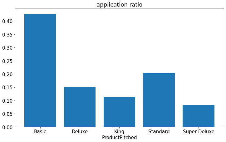
- 그래프를 통해 영업사원이 Basic 상품을 추천했을때 가장 신청률이 높은 것을 알 수 있다.
1.2.5.MaritalStatus ~ target
train_nona['MaritalStatus'].value_counts()
Married      949
Divorced     375
Single       349
Unmarried    282
Name: MaritalStatus, dtype: int64
train_enc['MaritalStatus'].value_counts()
1    949
0    375
2    349
3    282
Name: MaritalStatus, dtype: int64
fig=plt.figure(figsize=(10,10), dpi=100)
(ax1, ax2,ax3,ax4)=fig.subplots(1,4).flatten()

temp = train_enc[train_enc['MaritalStatus']==0].reset_index(drop = True)
x = temp['ProdTaken'].value_counts()
x.plot.pie(ax=ax1)
_=ax1.set_title('Divorced')


temp = train_enc[train_enc['MaritalStatus']==1].reset_index(drop = True)
x = temp['ProdTaken'].value_counts()
x.plot.pie(ax=ax2)
_=ax2.set_title('Married')

temp = train_enc[train_enc['MaritalStatus']==2].reset_index(drop = True)
x = temp['ProdTaken'].value_counts()
x.plot.pie(ax=ax3)
_=ax3.set_title('Single')

temp = train_enc[train_enc['MaritalStatus']==3].reset_index(drop = True)
x = temp['ProdTaken'].value_counts()
x.plot.pie(ax=ax4)
_=ax4.set_title('Unmarried')
ax4.legend(bbox_to_anchor=(0.9, 1), loc=2,labels=['no application','application'])
plt.show()
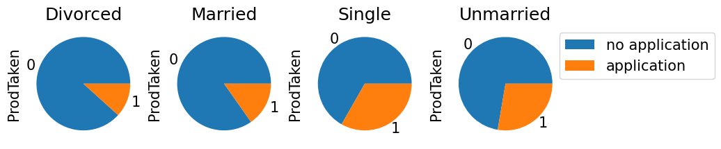
- Divorced 는 이혼한 사람을 뜻하는데 이혼한 사람과 결혼한 사람이 비슷한 신청률을 보였고, 미혼인 사람과 싱글인 사람이 25퍼센트가 넘는 신청률을 보였다.
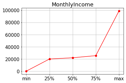
1.2.6.CityTier ~ MonthlyIncome
plt.rcParams['font.size'] = 15
data = train_enc.describe().loc['min':'max', 'MonthlyIncome']

plt.title('MonthlyIncome')
plt.plot(data, color = 'red', marker = 'o')
plt.grid(True)
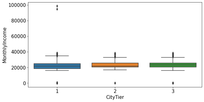
plt.figure(figsize=(10,5))
sns.boxplot(data=train_nona, x="CityTier", y="MonthlyIncome")
plt.show()
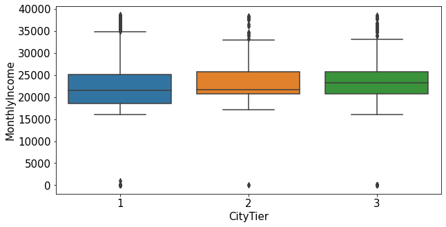
plt.figure(figsize=(10,5))
sns.boxplot(data=train_nona[train_nona['MonthlyIncome']<60000], x="CityTier", y="MonthlyIncome")
plt.show()
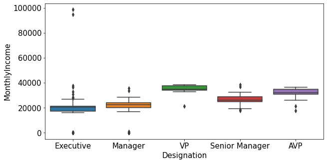
1.2.7.Designation ~ MonthlyIncome
plt.figure(figsize=(10,5))
sns.boxplot(data=train_nona, x="Designation", y="MonthlyIncome")
plt.show()
plt.figure(figsize=(10,5))
sns.boxplot(data=train_nona[train_nona['MonthlyIncome']<60000], x="Designation", y="MonthlyIncome")
plt.show()
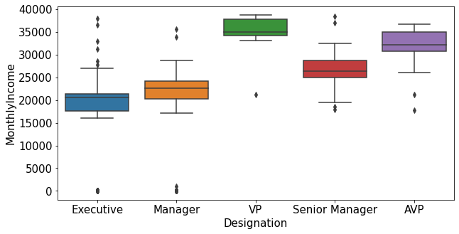
- MonthlyIncome의 이상치는 특정한 도시 등급과 직급에서 발견됨.
train_enc[train_enc['MonthlyIncome']>40000]['ProdTaken'].value_counts()
0    2
Name: ProdTaken, dtype: int64
1.2.8.NumberOfTrips ~ MonthlyIncome
plt.figure(figsize=(10,5))
sns.boxplot(data=train_nona, x="NumberOfTrips", y="MonthlyIncome")
plt.show()
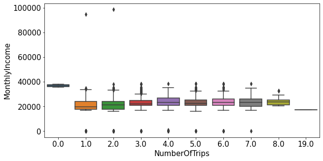
- 평균 연간 여행 횟수가 0인 사람들의 월 급여의 평균이 가장 높았다. 꼭 월 급여가 높다고 여행을 많이 다니는 것은 아닌 것을 알 수 있다.
1.2.9.DurationOfPitch ~ PitchSatisfactionScore
plt.figure(figsize=(10,5))
sns.boxplot(data=train_enc, x="PitchSatisfactionScore", y="DurationOfPitch")
plt.show()
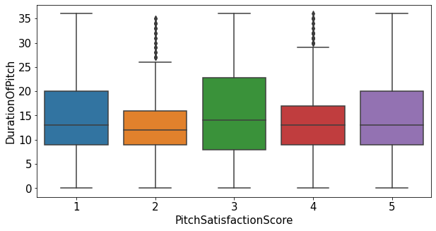
- 두 변수간 큰 상관관계가 없는 것으로 보임
1.2.10.heatmap
plt.figure(figsize=(15,15))
sns.heatmap(train_enc.corr(method='pearson'),annot=True, fmt='.1f', linewidths=.5, cmap='Blues')
<matplotlib.axes._subplots.AxesSubplot at 0x7fac6aeff410>
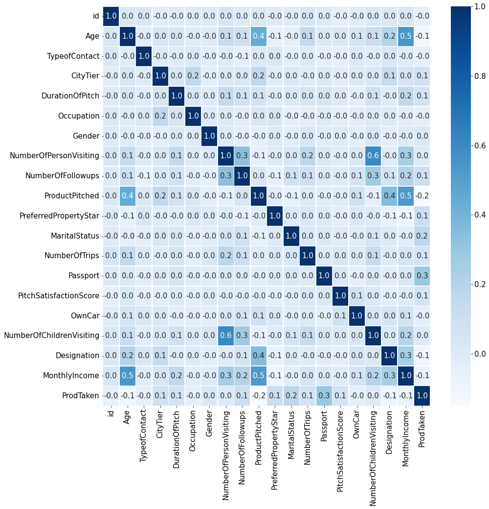
1.3.heatmap 정보를 기반으로 EDA
1.3.1. MonthlyIncome ~ Age
plt.figure(dpi=130)

sns.scatterplot(train_enc['Age'],train_enc['MonthlyIncome'])
plt.xlabel('Age')
plt.ylabel('MonthlyIncome')
plt.show()
/usr/local/lib/python3.7/dist-packages/seaborn/_decorators.py:43: FutureWarning: Pass the following variables as keyword args: x, y. From version 0.12, the only valid positional argument will be `data`, and passing other arguments without an explicit keyword will result in an error or misinterpretation.
  FutureWarning
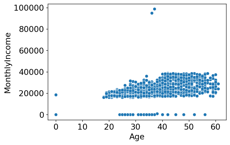
- 나이가 0인 데이터가 확인되고 또 그 중 월 급여가 0이 아닌 데이터가 보인다. 데이터의 오류가 아닐까 싶어 Age데이터를 확인해 봐야겠다.
train_enc[train_enc['Age']==0]
| id | Age | TypeofContact | CityTier | DurationOfPitch | Occupation | Gender | NumberOfPersonVisiting | NumberOfFollowups | ProductPitched | PreferredPropertyStar | MaritalStatus | NumberOfTrips | Passport | PitchSatisfactionScore | OwnCar | NumberOfChildrenVisiting | Designation | MonthlyIncome | ProdTaken | |
|---|---|---|---|---|---|---|---|---|---|---|---|---|---|---|---|---|---|---|---|---|
| 13 | 14 | 0.0 | 1 | 3 | 6.0 | 3 | 1 | 2 | 1.0 | 1 | 5.0 | 1 | 2.0 | 0 | 4 | 0 | 0.0 | 2 | 0.0 | 0 |
| 26 | 27 | 0.0 | 1 | 1 | 6.0 | 3 | 0 | 3 | 3.0 | 0 | 5.0 | 1 | 2.0 | 0 | 1 | 1 | 0.0 | 1 | 18591.0 | 0 |
| 35 | 36 | 0.0 | 1 | 2 | 14.0 | 2 | 1 | 2 | 3.0 | 1 | 4.0 | 1 | 3.0 | 0 | 3 | 1 | 1.0 | 2 | 0.0 | 0 |
| 87 | 88 | 0.0 | 1 | 2 | 8.0 | 2 | 1 | 3 | 3.0 | 0 | 3.0 | 2 | 1.0 | 0 | 1 | 0 | 0.0 | 1 | 18539.0 | 0 |
| 121 | 122 | 0.0 | 1 | 1 | 35.0 | 3 | 1 | 3 | 3.0 | 0 | 5.0 | 1 | 2.0 | 0 | 4 | 1 | 1.0 | 1 | 0.0 | 0 |
| ... | ... | ... | ... | ... | ... | ... | ... | ... | ... | ... | ... | ... | ... | ... | ... | ... | ... | ... | ... | ... |
| 1882 | 1883 | 0.0 | 1 | 1 | 15.0 | 2 | 1 | 1 | 4.0 | 0 | 3.0 | 2 | 1.0 | 0 | 2 | 1 | 0.0 | 1 | 0.0 | 0 |
| 1888 | 1889 | 0.0 | 1 | 1 | 12.0 | 3 | 0 | 3 | 4.0 | 1 | 3.0 | 2 | 2.0 | 1 | 4 | 1 | 1.0 | 2 | 0.0 | 0 |
| 1914 | 1915 | 0.0 | 1 | 1 | 7.0 | 2 | 0 | 3 | 3.0 | 0 | 3.0 | 1 | 2.0 | 0 | 1 | 1 | 2.0 | 1 | 0.0 | 0 |
| 1916 | 1917 | 0.0 | 1 | 2 | 26.0 | 3 | 0 | 3 | 3.0 | 0 | 4.0 | 1 | 1.0 | 1 | 3 | 0 | 1.0 | 1 | 18669.0 | 1 |
| 1923 | 1924 | 0.0 | 0 | 3 | 16.0 | 2 | 1 | 2 | 3.0 | 1 | 3.0 | 1 | 2.0 | 1 | 1 | 1 | 1.0 | 2 | 0.0 | 0 |
94 rows × 20 columns
test[test['Age']==0]
| id | Age | TypeofContact | CityTier | DurationOfPitch | Occupation | Gender | NumberOfPersonVisiting | NumberOfFollowups | ProductPitched | PreferredPropertyStar | MaritalStatus | NumberOfTrips | Passport | PitchSatisfactionScore | OwnCar | NumberOfChildrenVisiting | Designation | MonthlyIncome | |
|---|---|---|---|---|---|---|---|---|---|---|---|---|---|---|---|---|---|---|---|
| 20 | 21 | 0.0 | 1 | 1 | 8.0 | 3 | 1 | 2 | 5.0 | 0 | 3.0 | 1 | 6.0 | 1 | 3 | 1 | 1.0 | 1 | 18464.0 |
| 25 | 26 | 0.0 | 1 | 1 | 12.0 | 2 | 0 | 2 | 4.0 | 0 | 3.0 | 1 | 2.0 | 0 | 3 | 0 | 1.0 | 1 | 18702.0 |
| 54 | 55 | 0.0 | 1 | 1 | 6.0 | 3 | 1 | 2 | 3.0 | 0 | 4.0 | 1 | 2.0 | 0 | 3 | 0 | 0.0 | 1 | 0.0 |
| 67 | 68 | 0.0 | 1 | 1 | 6.0 | 3 | 1 | 3 | 3.0 | 0 | 4.0 | 1 | 2.0 | 0 | 5 | 0 | 1.0 | 1 | 0.0 |
| 95 | 96 | 0.0 | 0 | 1 | 15.0 | 2 | 1 | 2 | 3.0 | 1 | 3.0 | 1 | 4.0 | 0 | 3 | 1 | 0.0 | 2 | 0.0 |
| ... | ... | ... | ... | ... | ... | ... | ... | ... | ... | ... | ... | ... | ... | ... | ... | ... | ... | ... | ... |
| 2799 | 2800 | 0.0 | 1 | 1 | 8.0 | 3 | 1 | 2 | 5.0 | 0 | 3.0 | 0 | 6.0 | 1 | 3 | 1 | 0.0 | 1 | 18464.0 |
| 2811 | 2812 | 0.0 | 1 | 1 | 13.0 | 2 | 1 | 3 | 1.0 | 0 | 5.0 | 2 | 1.0 | 0 | 1 | 1 | 0.0 | 1 | 18578.0 |
| 2834 | 2835 | 0.0 | 1 | 3 | 14.0 | 3 | 1 | 2 | 3.0 | 0 | 4.0 | 1 | 1.0 | 0 | 1 | 0 | 1.0 | 1 | 0.0 |
| 2841 | 2842 | 0.0 | 0 | 1 | 22.0 | 2 | 0 | 3 | 5.0 | 0 | 5.0 | 2 | 2.0 | 1 | 4 | 0 | 0.0 | 1 | 0.0 |
| 2916 | 2917 | 0.0 | 1 | 1 | 11.0 | 3 | 1 | 2 | 4.0 | 1 | 3.0 | 1 | 2.0 | 0 | 4 | 1 | 1.0 | 2 | 0.0 |
132 rows × 19 columns
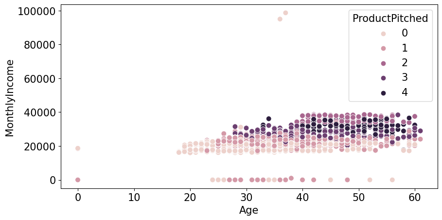
plt.figure(figsize=(10,5),dpi=100)

sns.scatterplot(train_enc['Age'],train_enc['MonthlyIncome'],hue=train_enc['ProductPitched'],s=60)
plt.xlabel('Age')
plt.ylabel('MonthlyIncome')

plt.legend(title='ProductPitched',loc='upper right')
plt.show()
/usr/local/lib/python3.7/dist-packages/seaborn/_decorators.py:43: FutureWarning: Pass the following variables as keyword args: x, y. From version 0.12, the only valid positional argument will be `data`, and passing other arguments without an explicit keyword will result in an error or misinterpretation.
  FutureWarning
1.3.1.1.Age가 0인 데이터 age 예측
- age가 0일 수는 없다고 생각해서 다른 feature들로 age를 예측해봐야겠다고 생각했다.
temp = train_enc[train_enc['Age']!=0]
temp
| id | Age | TypeofContact | CityTier | DurationOfPitch | Occupation | Gender | NumberOfPersonVisiting | NumberOfFollowups | ProductPitched | PreferredPropertyStar | MaritalStatus | NumberOfTrips | Passport | PitchSatisfactionScore | OwnCar | NumberOfChildrenVisiting | Designation | MonthlyIncome | ProdTaken | |
|---|---|---|---|---|---|---|---|---|---|---|---|---|---|---|---|---|---|---|---|---|
| 0 | 1 | 28.0 | 0 | 1 | 10.0 | 3 | 1 | 3 | 4.0 | 0 | 3.0 | 1 | 3.0 | 0 | 1 | 0 | 1.0 | 1 | 20384.0 | 0 |
| 1 | 2 | 34.0 | 1 | 3 | 0.0 | 3 | 0 | 2 | 4.0 | 1 | 4.0 | 2 | 1.0 | 1 | 5 | 1 | 0.0 | 2 | 19599.0 | 1 |
| 2 | 3 | 45.0 | 0 | 1 | 0.0 | 2 | 1 | 2 | 3.0 | 1 | 4.0 | 1 | 2.0 | 0 | 4 | 1 | 0.0 | 2 | 0.0 | 0 |
| 3 | 4 | 29.0 | 0 | 1 | 7.0 | 3 | 1 | 3 | 5.0 | 0 | 4.0 | 1 | 3.0 | 0 | 4 | 0 | 1.0 | 1 | 21274.0 | 1 |
| 4 | 5 | 42.0 | 1 | 3 | 6.0 | 2 | 1 | 2 | 3.0 | 1 | 3.0 | 0 | 2.0 | 0 | 3 | 1 | 0.0 | 2 | 19907.0 | 0 |
| ... | ... | ... | ... | ... | ... | ... | ... | ... | ... | ... | ... | ... | ... | ... | ... | ... | ... | ... | ... | ... |
| 1950 | 1951 | 28.0 | 1 | 1 | 10.0 | 3 | 1 | 3 | 5.0 | 0 | 3.0 | 2 | 2.0 | 0 | 1 | 1 | 2.0 | 1 | 20723.0 | 0 |
| 1951 | 1952 | 41.0 | 1 | 3 | 8.0 | 2 | 0 | 3 | 3.0 | 4 | 5.0 | 0 | 1.0 | 0 | 5 | 1 | 1.0 | 0 | 31595.0 | 0 |
| 1952 | 1953 | 38.0 | 0 | 3 | 28.0 | 3 | 0 | 3 | 4.0 | 0 | 3.0 | 0 | 7.0 | 0 | 2 | 1 | 2.0 | 1 | 21651.0 | 0 |
| 1953 | 1954 | 28.0 | 1 | 3 | 30.0 | 3 | 0 | 3 | 5.0 | 1 | 3.0 | 1 | 3.0 | 0 | 1 | 1 | 2.0 | 2 | 22218.0 | 0 |
| 1954 | 1955 | 22.0 | 0 | 1 | 9.0 | 2 | 1 | 2 | 4.0 | 0 | 3.0 | 0 | 1.0 | 1 | 3 | 0 | 0.0 | 1 | 17853.0 | 1 |
1861 rows × 20 columns
features = temp.columns[2:-1]
target = 'Age'
from sklearn.ensemble import RandomForestRegressor
from sklearn.model_selection import train_test_split
from sklearn.metrics import mean_absolute_error

X = temp[features]
y = temp[target]

X_train,X_test,y_train,y_test = train_test_split(X,y,train_size=0.9,shuffle=False)
model_rf = RandomForestRegressor()

model_rf.fit(X_train,y_train)

predict = model_rf.predict(X_test)
y_test
1755    54.0
1756    59.0
1757    21.0
1758    43.0
1759    48.0
        ...
1950    28.0
1951    41.0
1952    38.0
1953    28.0
1954    22.0
Name: Age, Length: 187, dtype: float64
plt.figure(dpi=130)
plt.plot(predict)
plt.plot(y_test.values,alpha=0.7)
plt.show()
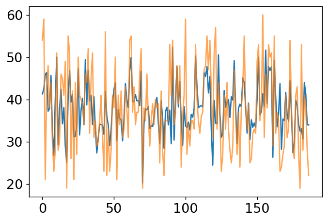
mean_absolute_error(predict,y_test)
5.528181818181818
temp = train_enc[train_enc['Age']==0]
temp
| id | Age | TypeofContact | CityTier | DurationOfPitch | Occupation | Gender | NumberOfPersonVisiting | NumberOfFollowups | ProductPitched | PreferredPropertyStar | MaritalStatus | NumberOfTrips | Passport | PitchSatisfactionScore | OwnCar | NumberOfChildrenVisiting | Designation | MonthlyIncome | ProdTaken | |
|---|---|---|---|---|---|---|---|---|---|---|---|---|---|---|---|---|---|---|---|---|
| 13 | 14 | 0.0 | 1 | 3 | 6.0 | 3 | 1 | 2 | 1.0 | 1 | 5.0 | 1 | 2.0 | 0 | 4 | 0 | 0.0 | 2 | 0.0 | 0 |
| 26 | 27 | 0.0 | 1 | 1 | 6.0 | 3 | 0 | 3 | 3.0 | 0 | 5.0 | 1 | 2.0 | 0 | 1 | 1 | 0.0 | 1 | 18591.0 | 0 |
| 35 | 36 | 0.0 | 1 | 2 | 14.0 | 2 | 1 | 2 | 3.0 | 1 | 4.0 | 1 | 3.0 | 0 | 3 | 1 | 1.0 | 2 | 0.0 | 0 |
| 87 | 88 | 0.0 | 1 | 2 | 8.0 | 2 | 1 | 3 | 3.0 | 0 | 3.0 | 2 | 1.0 | 0 | 1 | 0 | 0.0 | 1 | 18539.0 | 0 |
| 121 | 122 | 0.0 | 1 | 1 | 35.0 | 3 | 1 | 3 | 3.0 | 0 | 5.0 | 1 | 2.0 | 0 | 4 | 1 | 1.0 | 1 | 0.0 | 0 |
| ... | ... | ... | ... | ... | ... | ... | ... | ... | ... | ... | ... | ... | ... | ... | ... | ... | ... | ... | ... | ... |
| 1882 | 1883 | 0.0 | 1 | 1 | 15.0 | 2 | 1 | 1 | 4.0 | 0 | 3.0 | 2 | 1.0 | 0 | 2 | 1 | 0.0 | 1 | 0.0 | 0 |
| 1888 | 1889 | 0.0 | 1 | 1 | 12.0 | 3 | 0 | 3 | 4.0 | 1 | 3.0 | 2 | 2.0 | 1 | 4 | 1 | 1.0 | 2 | 0.0 | 0 |
| 1914 | 1915 | 0.0 | 1 | 1 | 7.0 | 2 | 0 | 3 | 3.0 | 0 | 3.0 | 1 | 2.0 | 0 | 1 | 1 | 2.0 | 1 | 0.0 | 0 |
| 1916 | 1917 | 0.0 | 1 | 2 | 26.0 | 3 | 0 | 3 | 3.0 | 0 | 4.0 | 1 | 1.0 | 1 | 3 | 0 | 1.0 | 1 | 18669.0 | 1 |
| 1923 | 1924 | 0.0 | 0 | 3 | 16.0 | 2 | 1 | 2 | 3.0 | 1 | 3.0 | 1 | 2.0 | 1 | 1 | 1 | 1.0 | 2 | 0.0 | 0 |
94 rows × 20 columns
X = temp[features]

train_enc.loc[train_enc['Age']==0,'Age'] = model_rf.predict(X)
train_enc['Age'].value_counts().sort_index()
18.0     5
19.0    16
20.0    13
21.0    17
22.0    20
        ..
57.0     9
58.0    11
59.0    14
60.0    12
61.0     3
Name: Age, Length: 135, dtype: int64
plt.figure(figsize=(10,5),dpi=100)

sns.scatterplot(train_enc['Age'],train_enc['MonthlyIncome'],hue=train_enc['ProductPitched'],s=60)
plt.xlabel('Age')
plt.ylabel('MonthlyIncome')

plt.legend(title='ProductPitched',loc='upper right')
plt.show()
/usr/local/lib/python3.7/dist-packages/seaborn/_decorators.py:43: FutureWarning: Pass the following variables as keyword args: x, y. From version 0.12, the only valid positional argument will be `data`, and passing other arguments without an explicit keyword will result in an error or misinterpretation.
  FutureWarning
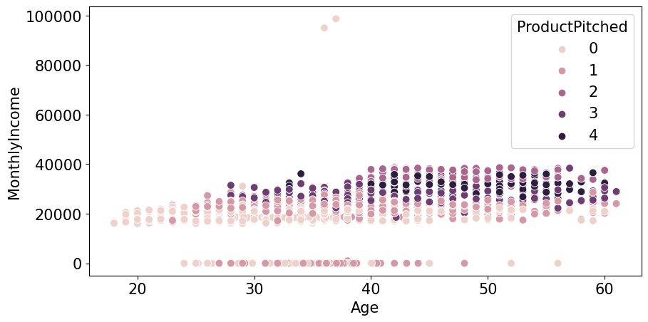
- Age 가 0인 데이터가 없어진 것을 확인 할 수있다.
1.3.2.MonthlyIncome ~ NumberOfPersonVisiting
train_enc['NumberOfPersonVisiting'].value_counts()
3    988
2    543
4    412
1     11
5      1
Name: NumberOfPersonVisiting, dtype: int64
temp = train_enc['NumberOfPersonVisiting'].value_counts()

plt.figure(dpi=100)

plt.bar(temp.index,temp.values)
plt.xlabel('NumberOfPersonVisiting')
plt.ylabel('counts')
plt.show()
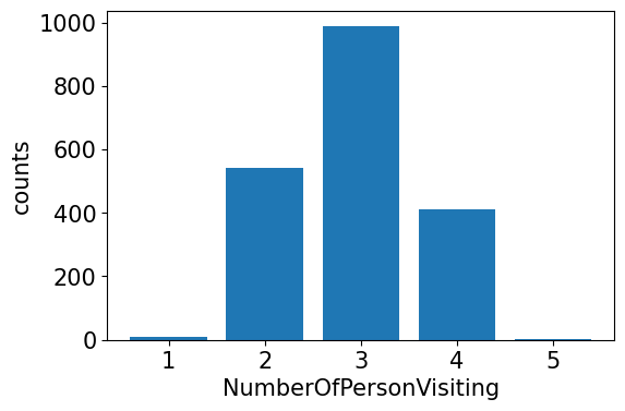
- 혼자 가거나 5명이서 가는 경우는 거의 없고 2,3,4명이서 가는 경우가 많다
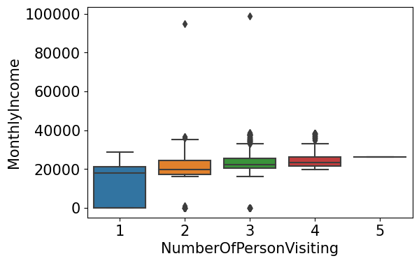
plt.figure(dpi=100)
sns.boxplot(data=train_enc, x="NumberOfPersonVisiting", y="MonthlyIncome")
plt.show()
plt.figure(dpi=100)
sns.violinplot(data=train_enc, x="NumberOfPersonVisiting", y="MonthlyIncome")
plt.show()
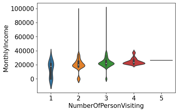
- 2,3,4 에는 차이가 크지 않지만 확실히 혼자가는 사람은 월 급여가 낮은 것을 알 수 있다.
1.3.3.MonthlyIncome ~ DurationOfPitch
train_enc['DurationOfPitch'].value_counts()
9.0     199
7.0     126
8.0     122
6.0     116
16.0    114
14.0    112
15.0    105
10.0    103
0.0     102
12.0     85
11.0     83
13.0     83
17.0     75
23.0     41
30.0     39
22.0     36
31.0     34
25.0     32
27.0     31
32.0     30
20.0     29
35.0     29
26.0     27
29.0     27
24.0     27
28.0     25
21.0     24
18.0     23
33.0     22
19.0     18
34.0     18
36.0     15
5.0       3
Name: DurationOfPitch, dtype: int64
plt.figure(dpi=130)

sns.scatterplot(train_enc['DurationOfPitch'],train_enc['MonthlyIncome'])
plt.xlabel('DurationOfPitch')
plt.ylabel('MonthlyIncome')
plt.show()
/usr/local/lib/python3.7/dist-packages/seaborn/_decorators.py:43: FutureWarning: Pass the following variables as keyword args: x, y. From version 0.12, the only valid positional argument will be `data`, and passing other arguments without an explicit keyword will result in an error or misinterpretation.
  FutureWarning
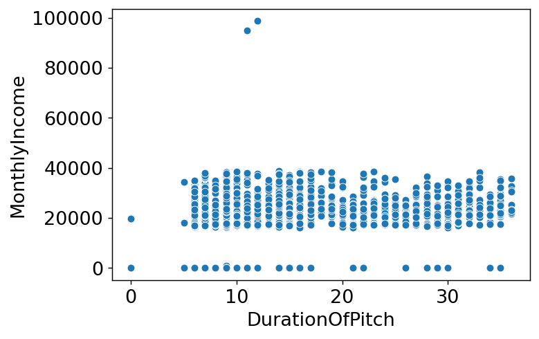
- 상관관계를 찾기 힘들어보임.
2.Feature engineering
plt.figure(figsize=(15,15))
sns.heatmap(train_enc.corr(method='pearson'),annot=True, fmt='.1f', linewidths=.5, cmap='Blues')
<matplotlib.axes._subplots.AxesSubplot at 0x7fac6aa35410>
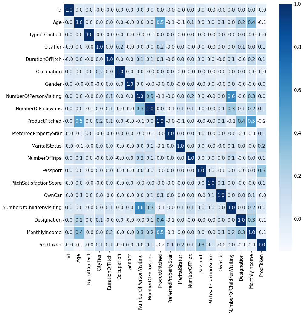
- 새로운 파생변수를 만들고 싶지만 데이터의 타입이 대부분 카테고리형태여서 힘들 것 같다.
2.1.drop
- target과 상관관계가 낮은 feature는 설정X
train_enc.corr()['ProdTaken']
id                         -0.048933
Age                        -0.136257
TypeofContact              -0.047598
CityTier                    0.085583
DurationOfPitch             0.069795
Occupation                 -0.042101
Gender                      0.019991
NumberOfPersonVisiting      0.006483
NumberOfFollowups           0.102778
ProductPitched             -0.150399
PreferredPropertyStar       0.108886
MaritalStatus               0.169245
NumberOfTrips               0.060995
Passport                    0.293726
PitchSatisfactionScore      0.067736
OwnCar                     -0.040465
NumberOfChildrenVisiting    0.010089
Designation                -0.096041
MonthlyIncome              -0.077508
ProdTaken                   1.000000
Name: ProdTaken, dtype: float64
train_enc.corr()['ProdTaken'].index
Index(['id', 'Age', 'TypeofContact', 'CityTier', 'DurationOfPitch',
       'Occupation', 'Gender', 'NumberOfPersonVisiting', 'NumberOfFollowups',
       'ProductPitched', 'PreferredPropertyStar', 'MaritalStatus',
       'NumberOfTrips', 'Passport', 'PitchSatisfactionScore', 'OwnCar',
       'NumberOfChildrenVisiting', 'Designation', 'MonthlyIncome',
       'ProdTaken'],
      dtype='object')
features = ['Age','CityTier', 'DurationOfPitch',
       'Occupation',  'NumberOfFollowups',
       'ProductPitched', 'PreferredPropertyStar', 'MaritalStatus',
       'NumberOfTrips', 'Passport', 'PitchSatisfactionScore', 'OwnCar',
        'Designation', 'MonthlyIncome',
       'ProdTaken']
features
['Age',
 'CityTier',
 'DurationOfPitch',
 'Occupation',
 'NumberOfFollowups',
 'ProductPitched',
 'PreferredPropertyStar',
 'MaritalStatus',
 'NumberOfTrips',
 'Passport',
 'PitchSatisfactionScore',
 'OwnCar',
 'Designation',
 'MonthlyIncome',
 'ProdTaken']
2.2.scaling
train_enc.head()
| id | Age | TypeofContact | CityTier | DurationOfPitch | Occupation | Gender | NumberOfPersonVisiting | NumberOfFollowups | ProductPitched | PreferredPropertyStar | MaritalStatus | NumberOfTrips | Passport | PitchSatisfactionScore | OwnCar | NumberOfChildrenVisiting | Designation | MonthlyIncome | ProdTaken | |
|---|---|---|---|---|---|---|---|---|---|---|---|---|---|---|---|---|---|---|---|---|
| 0 | 1 | 28.0 | 0 | 1 | 10.0 | 3 | 1 | 3 | 4.0 | 0 | 3.0 | 1 | 3.0 | 0 | 1 | 0 | 1.0 | 1 | 20384.0 | 0 |
| 1 | 2 | 34.0 | 1 | 3 | 0.0 | 3 | 0 | 2 | 4.0 | 1 | 4.0 | 2 | 1.0 | 1 | 5 | 1 | 0.0 | 2 | 19599.0 | 1 |
| 2 | 3 | 45.0 | 0 | 1 | 0.0 | 2 | 1 | 2 | 3.0 | 1 | 4.0 | 1 | 2.0 | 0 | 4 | 1 | 0.0 | 2 | 0.0 | 0 |
| 3 | 4 | 29.0 | 0 | 1 | 7.0 | 3 | 1 | 3 | 5.0 | 0 | 4.0 | 1 | 3.0 | 0 | 4 | 0 | 1.0 | 1 | 21274.0 | 1 |
| 4 | 5 | 42.0 | 1 | 3 | 6.0 | 2 | 1 | 2 | 3.0 | 1 | 3.0 | 0 | 2.0 | 0 | 3 | 1 | 0.0 | 2 | 19907.0 | 0 |
from sklearn.preprocessing import StandardScaler

scaler = StandardScaler()

train_enc[['MonthlyIncome']] = scaler.fit_transform(train_enc[['MonthlyIncome']])
train_enc.head()
| id | Age | TypeofContact | CityTier | DurationOfPitch | Occupation | Gender | NumberOfPersonVisiting | NumberOfFollowups | ProductPitched | PreferredPropertyStar | MaritalStatus | NumberOfTrips | Passport | PitchSatisfactionScore | OwnCar | NumberOfChildrenVisiting | Designation | MonthlyIncome | ProdTaken | |
|---|---|---|---|---|---|---|---|---|---|---|---|---|---|---|---|---|---|---|---|---|
| 0 | 1 | 28.0 | 0 | 1 | 10.0 | 3 | 1 | 3 | 4.0 | 0 | 3.0 | 1 | 3.0 | 0 | 1 | 0 | 1.0 | 1 | -0.268499 | 0 |
| 1 | 2 | 34.0 | 1 | 3 | 0.0 | 3 | 0 | 2 | 4.0 | 1 | 4.0 | 2 | 1.0 | 1 | 5 | 1 | 0.0 | 2 | -0.372240 | 1 |
| 2 | 3 | 45.0 | 0 | 1 | 0.0 | 2 | 1 | 2 | 3.0 | 1 | 4.0 | 1 | 2.0 | 0 | 4 | 1 | 0.0 | 2 | -2.962326 | 0 |
| 3 | 4 | 29.0 | 0 | 1 | 7.0 | 3 | 1 | 3 | 5.0 | 0 | 4.0 | 1 | 3.0 | 0 | 4 | 0 | 1.0 | 1 | -0.150882 | 1 |
| 4 | 5 | 42.0 | 1 | 3 | 6.0 | 2 | 1 | 2 | 3.0 | 1 | 3.0 | 0 | 2.0 | 0 | 3 | 1 | 0.0 | 2 | -0.331537 | 0 |
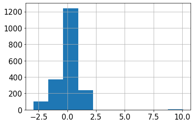
train_enc['MonthlyIncome'].hist()
<matplotlib.axes._subplots.AxesSubplot at 0x7fac6ad5add0>
3.모델링을 위한 데이터 전처리
0.1.3.(추가) 결측치 처리 모듈 생성
- 0으로 채운 수치형 컬럼의 결측치를 회귀예측 모델로 예측하여 채워넣는 모듈 생성
from sklearn.ensemble import RandomForestRegressor
from sklearn.model_selection import train_test_split
from sklearn.metrics import mean_absolute_error
from sklearn.ensemble import ExtraTreesRegressor
def prod_val(feature:str):
  if len(train_enc[train_enc[feature]==0])==0:
    return 'already processed'
  train_temp = train_enc[train_enc[feature]!=0]

  features = train_temp.columns[1:-1].drop(feature)
  target = feature

  X = train_temp[features]
  y = train_temp[target]

  X_train,X_test,y_train,y_test = train_test_split(X,y,train_size=0.9,shuffle=False)
  model_rf = ExtraTreesRegressor(n_estimators=300)

  model_rf.fit(X_train,y_train)

  train_predict = model_rf.predict(X_test)

  print(f'{feature} MAE: {mean_absolute_error(train_predict,y_test)}')

  X = train_enc[train_enc[feature]==0][features]

  train_enc.loc[train_enc[feature]==0,feature] = model_rf.predict(X)

  test_temp = test[test[feature]==0]

  X = test_temp[features]

  test.loc[test[feature]==0,feature] = model_rf.predict(X)

  print(f'\ntrain set: \n{train_enc[feature].value_counts().sort_index().head(3)}')
  print(f'\ntest set: \n{test[feature].value_counts().sort_index().head(3)}')
train = pd.read_csv('/content/drive/MyDrive/data/여행상품신청/train.csv')
test = pd.read_csv('/content/drive/MyDrive/data/여행상품신청/test.csv')
sample_submission = pd.read_csv('/content/drive/MyDrive/data/여행상품신청/sample_submission.csv')
3.1.결측치 처리
def handle_na(data):
    temp = data.copy()
    for col, dtype in temp.dtypes.items():
        if dtype == 'object':
            # 문자형 칼럼의 경우 'Unknown'을 채워줍니다.
            value = 'Unknown'
        elif dtype == int or dtype == float:
            # 수치형 칼럼의 경우 0을 채워줍니다.
            value = 0
        temp.loc[:,col] = temp[col].fillna(value)
    return temp

train_nona = handle_na(train)

# 결측치 처리가 잘 되었는지 확인해 줍니다.
train_nona.isna().sum()
id                          0
Age                         0
TypeofContact               0
CityTier                    0
DurationOfPitch             0
Occupation                  0
Gender                      0
NumberOfPersonVisiting      0
NumberOfFollowups           0
ProductPitched              0
PreferredPropertyStar       0
MaritalStatus               0
NumberOfTrips               0
Passport                    0
PitchSatisfactionScore      0
OwnCar                      0
NumberOfChildrenVisiting    0
Designation                 0
MonthlyIncome               0
ProdTaken                   0
dtype: int64
3.2.문자형 변수 전처리
train_nona.loc[train_nona['Gender']=='Fe Male','Gender'] = 'Female'
test.loc[test['Gender']=='Fe Male','Gender'] = 'Female'
train_nona['Gender'].value_counts()
Male      1207
Female     748
Name: Gender, dtype: int64
# LabelEncoder를 준비해줍니다.
from sklearn.preprocessing import LabelEncoder

encoder = LabelEncoder()

# LabelEcoder는 학습하는 과정을 필요로 합니다.
encoder.fit(train_nona['TypeofContact'])

#학습된 encoder를 사용하여 문자형 변수를 숫자로 변환해줍니다.
encoder.transform(train_nona['TypeofContact'])
array([0, 1, 0, ..., 0, 1, 0])
train_enc = train_nona.copy()
object_columns = train_nona.columns[train_nona.dtypes == 'object']
# 모든 문자형 변수에 대해 encoder를 적용합니다.
for o_col in object_columns:
    encoder = LabelEncoder()
    encoder.fit(train_enc[o_col])
    train_enc[o_col] = encoder.transform(train_enc[o_col])

# 결과를 확인합니다.
train_enc
| id | Age | TypeofContact | CityTier | DurationOfPitch | Occupation | Gender | NumberOfPersonVisiting | NumberOfFollowups | ProductPitched | PreferredPropertyStar | MaritalStatus | NumberOfTrips | Passport | PitchSatisfactionScore | OwnCar | NumberOfChildrenVisiting | Designation | MonthlyIncome | ProdTaken | |
|---|---|---|---|---|---|---|---|---|---|---|---|---|---|---|---|---|---|---|---|---|
| 0 | 1 | 28.0 | 0 | 1 | 10.0 | 3 | 1 | 3 | 4.0 | 0 | 3.0 | 1 | 3.0 | 0 | 1 | 0 | 1.0 | 1 | 20384.0 | 0 |
| 1 | 2 | 34.0 | 1 | 3 | 0.0 | 3 | 0 | 2 | 4.0 | 1 | 4.0 | 2 | 1.0 | 1 | 5 | 1 | 0.0 | 2 | 19599.0 | 1 |
| 2 | 3 | 45.0 | 0 | 1 | 0.0 | 2 | 1 | 2 | 3.0 | 1 | 4.0 | 1 | 2.0 | 0 | 4 | 1 | 0.0 | 2 | 0.0 | 0 |
| 3 | 4 | 29.0 | 0 | 1 | 7.0 | 3 | 1 | 3 | 5.0 | 0 | 4.0 | 1 | 3.0 | 0 | 4 | 0 | 1.0 | 1 | 21274.0 | 1 |
| 4 | 5 | 42.0 | 1 | 3 | 6.0 | 2 | 1 | 2 | 3.0 | 1 | 3.0 | 0 | 2.0 | 0 | 3 | 1 | 0.0 | 2 | 19907.0 | 0 |
| ... | ... | ... | ... | ... | ... | ... | ... | ... | ... | ... | ... | ... | ... | ... | ... | ... | ... | ... | ... | ... |
| 1950 | 1951 | 28.0 | 1 | 1 | 10.0 | 3 | 1 | 3 | 5.0 | 0 | 3.0 | 2 | 2.0 | 0 | 1 | 1 | 2.0 | 1 | 20723.0 | 0 |
| 1951 | 1952 | 41.0 | 1 | 3 | 8.0 | 2 | 0 | 3 | 3.0 | 4 | 5.0 | 0 | 1.0 | 0 | 5 | 1 | 1.0 | 0 | 31595.0 | 0 |
| 1952 | 1953 | 38.0 | 0 | 3 | 28.0 | 3 | 0 | 3 | 4.0 | 0 | 3.0 | 0 | 7.0 | 0 | 2 | 1 | 2.0 | 1 | 21651.0 | 0 |
| 1953 | 1954 | 28.0 | 1 | 3 | 30.0 | 3 | 0 | 3 | 5.0 | 1 | 3.0 | 1 | 3.0 | 0 | 1 | 1 | 2.0 | 2 | 22218.0 | 0 |
| 1954 | 1955 | 22.0 | 0 | 1 | 9.0 | 2 | 1 | 2 | 4.0 | 0 | 3.0 | 0 | 1.0 | 1 | 3 | 0 | 0.0 | 1 | 17853.0 | 1 |
1955 rows × 20 columns
# 결측치 처리
test = handle_na(test)

# 문자형 변수 전처리
for o_col in object_columns:
    encoder = LabelEncoder()

    # test 데이터를 이용해 encoder를 학습하는 것은 Data Leakage 입니다! 조심!
    encoder.fit(train_nona[o_col])

    # test 데이터는 오로지 transform 에서만 사용되어야 합니다.
    test[o_col] = encoder.transform(test[o_col])

# 결과를 확인합니다.
test
| id | Age | TypeofContact | CityTier | DurationOfPitch | Occupation | Gender | NumberOfPersonVisiting | NumberOfFollowups | ProductPitched | PreferredPropertyStar | MaritalStatus | NumberOfTrips | Passport | PitchSatisfactionScore | OwnCar | NumberOfChildrenVisiting | Designation | MonthlyIncome | |
|---|---|---|---|---|---|---|---|---|---|---|---|---|---|---|---|---|---|---|---|
| 0 | 1 | 32.0 | 0 | 3 | 0.0 | 3 | 1 | 2 | 5.0 | 1 | 3.0 | 1 | 1.0 | 0 | 2 | 0 | 1.0 | 2 | 19668.0 |
| 1 | 2 | 46.0 | 1 | 2 | 11.0 | 3 | 1 | 3 | 0.0 | 1 | 4.0 | 1 | 1.0 | 1 | 5 | 0 | 1.0 | 2 | 20021.0 |
| 2 | 3 | 37.0 | 1 | 3 | 22.0 | 3 | 1 | 3 | 4.0 | 1 | 3.0 | 1 | 5.0 | 0 | 5 | 1 | 0.0 | 2 | 21334.0 |
| 3 | 4 | 43.0 | 1 | 1 | 36.0 | 3 | 1 | 3 | 6.0 | 1 | 3.0 | 3 | 6.0 | 0 | 3 | 1 | 2.0 | 2 | 22950.0 |
| 4 | 5 | 25.0 | 1 | 3 | 7.0 | 1 | 0 | 4 | 4.0 | 0 | 4.0 | 3 | 3.0 | 1 | 4 | 1 | 3.0 | 1 | 21880.0 |
| ... | ... | ... | ... | ... | ... | ... | ... | ... | ... | ... | ... | ... | ... | ... | ... | ... | ... | ... | ... |
| 2928 | 2929 | 54.0 | 1 | 1 | 6.0 | 3 | 0 | 2 | 3.0 | 4 | 3.0 | 2 | 7.0 | 0 | 4 | 1 | 1.0 | 0 | 32328.0 |
| 2929 | 2930 | 33.0 | 1 | 1 | 9.0 | 3 | 0 | 4 | 2.0 | 1 | 3.0 | 3 | 2.0 | 0 | 3 | 0 | 1.0 | 2 | 23733.0 |
| 2930 | 2931 | 33.0 | 0 | 1 | 31.0 | 2 | 1 | 4 | 4.0 | 1 | 3.0 | 0 | 3.0 | 0 | 4 | 1 | 1.0 | 2 | 23987.0 |
| 2931 | 2932 | 26.0 | 1 | 1 | 9.0 | 3 | 1 | 4 | 2.0 | 0 | 5.0 | 3 | 2.0 | 0 | 2 | 1 | 3.0 | 1 | 22102.0 |
| 2932 | 2933 | 31.0 | 1 | 1 | 9.0 | 2 | 1 | 3 | 5.0 | 1 | 3.0 | 0 | 3.0 | 0 | 4 | 1 | 1.0 | 2 | 22830.0 |
2933 rows × 19 columns
3.3.결측치 처리 모듈 적용
prod_val('Age')
Age MAE: 5.071390374331551

train set:
18.0     5
19.0    16
20.0    13
Name: Age, dtype: int64

test set:
18.0     9
19.0    16
20.0    25
Name: Age, dtype: int64
train_enc['Age'] = train_enc['Age'].round()
test['Age'] = test['Age'].round()
train_enc['Age'].unique()
array([28., 34., 45., 29., 42., 32., 43., 36., 35., 31., 49., 33., 52.,
       22., 50., 23., 41., 37., 40., 56., 54., 39., 20., 38., 46., 27.,
       25., 26., 24., 30., 21., 51., 47., 55., 44., 53., 48., 18., 57.,
       60., 59., 19., 58., 61.])
prod_val('MonthlyIncome')
MonthlyIncome MAE: 1205.1359677419355

train set:
1000.00     1
14781.04    1
16009.00    1
Name: MonthlyIncome, dtype: int64

test set:
2196.853333     1
4678.000000     1
14921.480000    1
Name: MonthlyIncome, dtype: int64
prod_val('DurationOfPitch')
DurationOfPitch MAE: 6.203512544802866

train set:
5.0      3
6.0    116
7.0    126
Name: DurationOfPitch, dtype: int64

test set:
5.0      3
6.0    191
7.0    216
Name: DurationOfPitch, dtype: int64
train_enc['DurationOfPitch'] = train_enc['DurationOfPitch'].round()
test['DurationOfPitch'] = test['DurationOfPitch'].round()
test['DurationOfPitch'].unique()
array([ 16.,  11.,  22.,  36.,   7.,   8.,   6.,  29.,   9.,  12.,  13.,
        17.,  15.,  10.,  14.,  35.,  24.,  31.,  21.,  19.,  32.,  27.,
        18.,  33.,  30.,  26.,  34.,  23.,  20.,  28.,  25., 126.,   5.,
       127.])
prod_val('NumberOfTrips')
NumberOfTrips MAE: 1.2843333333333333

train set:
1.000000    234
1.963333      1
2.000000    594
Name: NumberOfTrips, dtype: int64

test set:
1.000000    386
2.000000    870
2.856667      1
Name: NumberOfTrips, dtype: int64
train_enc['NumberOfTrips'] = train_enc['NumberOfTrips'].round()
test['NumberOfTrips'] = test['NumberOfTrips'].round()
test['NumberOfTrips'].unique()
array([ 1., 5., 6., 3., 7., 4., 2., 8., 22., 21., 20.])
prod_val('NumberOfFollowups')
NumberOfFollowups MAE: 0.605094017094017

train set:
1.000000    74
2.000000    89
2.436667     1
Name: NumberOfFollowups, dtype: int64

test set:
1.000000    102
2.000000    140
2.706667      1
Name: NumberOfFollowups, dtype: int64
train_enc['NumberOfFollowups'] = train_enc['NumberOfFollowups'].round()
test['NumberOfFollowups'] = test['NumberOfFollowups'].round()
test['NumberOfFollowups'].unique()
array([5., 3., 4., 6., 1., 2.])
prod_val('PreferredPropertyStar')
PreferredPropertyStar MAE: 0.6105299145299146

train set:
3.000000    1212
3.126667       1
3.353333       1
Name: PreferredPropertyStar, dtype: int64

test set:
3.000000    1781
3.033333       1
3.100000       1
Name: PreferredPropertyStar, dtype: int64
train_enc['PreferredPropertyStar'] = train_enc['PreferredPropertyStar'].round()
test['PreferredPropertyStar'] = test['PreferredPropertyStar'].round()
test['PreferredPropertyStar'].unique()
array([3., 4., 5.])
prod_val('NumberOfChildrenVisiting')
NumberOfChildrenVisiting MAE: 0.5187938596491228

train set:
1.000000    1099
1.003333       6
1.030000       1
Name: NumberOfChildrenVisiting, dtype: int64

test set:
1.000000    1712
1.003333       3
1.043333       1
Name: NumberOfChildrenVisiting, dtype: int64
train_enc['NumberOfChildrenVisiting'] = train_enc['NumberOfChildrenVisiting'].round()
test['NumberOfChildrenVisiting'] = test['NumberOfChildrenVisiting'].round()
test['NumberOfChildrenVisiting'].unique()
array([1., 2., 3.])
3.3.(모듈대체) Age가 0인 데이터 age 예측
- age의 결측치를 0으로 채웠었는데 다른 feature들로 age를 예측해봐야겠다고 생각했다.
# temp = train_enc[train_enc['Age']!=0]
# temp.head()
# features = temp.columns[2:-1]
# target = 'Age'
# from sklearn.ensemble import RandomForestRegressor
# from sklearn.model_selection import train_test_split
# from sklearn.metrics import mean_absolute_error

# X = temp[features]
# y = temp[target]

# X_train,X_test,y_train,y_test = train_test_split(X,y,train_size=0.9,shuffle=False)
# model_rf = ExtraTreesRegressor(n_estimators=500)

# model_rf.fit(X_train,y_train)

# predict = model_rf.predict(X_test)
# mean_absolute_error(predict,y_test)
# temp = train_enc[train_enc['Age']==0]
# temp.head()
# X = temp[features]

# train_enc.loc[train_enc['Age']==0,'Age'] = model_rf.predict(X)
# train_enc['Age'].value_counts().sort_index()
# temp = test[test['Age']==0]
# temp.head()
# X = temp[features]

# test.loc[test['Age']==0,'Age'] = model_rf.predict(X)
# test['Age'].value_counts().sort_index()
3.4.(모듈대체) Monthly Income 결측치 예측
- Age와 같은 방법으로 Monthly Income을 예측해보자
# temp = train_enc[train_enc['MonthlyIncome']!=0]
# temp.head()
# features = temp.columns[1:-1].drop('MonthlyIncome')
# target = 'MonthlyIncome'
# features
# from sklearn.ensemble import ExtraTreesRegressor

# X = temp[features]
# y = temp[target]

# X_train,X_test,y_train,y_test = train_test_split(X,y,train_size=0.9,shuffle=False)
# model_rf = ExtraTreesRegressor(n_estimators=500)

# model_rf.fit(X_train,y_train)

# predict = model_rf.predict(X_test)
# mean_absolute_error(predict,y_test)
# temp = train_enc[train_enc['MonthlyIncome']==0]
# temp.head()
# X = temp[features]

# train_enc.loc[train_enc['MonthlyIncome']==0,'MonthlyIncome'] = model_rf.predict(X)
# train_enc['MonthlyIncome'].value_counts().sort_index()
# temp = test[test['MonthlyIncome']==0]
# temp.head()
# X = temp[features]

# test.loc[test['MonthlyIncome']==0,'MonthlyIncome'] = model_rf.predict(X)
# test['MonthlyIncome'].value_counts().sort_index()
3.4.scaling
from sklearn.preprocessing import StandardScaler
from sklearn.preprocessing import MinMaxScaler

scaler = StandardScaler()
min_scaler = MinMaxScaler()

train_enc[['MonthlyIncome']] = scaler.fit_transform(train_enc[['MonthlyIncome']])
test[['MonthlyIncome']] = scaler.transform(test[['MonthlyIncome']])

train_enc[['Age','DurationOfPitch']] = min_scaler.fit_transform(train_enc[['Age','DurationOfPitch']])
test[['Age','DurationOfPitch']] = min_scaler.transform(test[['Age','DurationOfPitch']])

train_enc.head()
| id | Age | TypeofContact | CityTier | DurationOfPitch | Occupation | Gender | NumberOfPersonVisiting | NumberOfFollowups | ProductPitched | PreferredPropertyStar | MaritalStatus | NumberOfTrips | Passport | PitchSatisfactionScore | OwnCar | NumberOfChildrenVisiting | Designation | MonthlyIncome | ProdTaken | |
|---|---|---|---|---|---|---|---|---|---|---|---|---|---|---|---|---|---|---|---|---|
| 0 | 1 | 0.232558 | 0 | 1 | 0.161290 | 3 | 1 | 3 | 4.0 | 0 | 3.0 | 1 | 3.0 | 0 | 1 | 0 | 1.0 | 1 | -0.543896 | 0 |
| 1 | 2 | 0.372093 | 1 | 3 | 0.516129 | 3 | 0 | 2 | 4.0 | 1 | 4.0 | 2 | 1.0 | 1 | 5 | 1 | 1.0 | 2 | -0.684698 | 1 |
| 2 | 3 | 0.627907 | 0 | 1 | 0.322581 | 2 | 1 | 2 | 3.0 | 1 | 4.0 | 1 | 2.0 | 0 | 4 | 1 | 1.0 | 2 | -0.697951 | 0 |
| 3 | 4 | 0.255814 | 0 | 1 | 0.064516 | 3 | 1 | 3 | 5.0 | 0 | 4.0 | 1 | 3.0 | 0 | 4 | 0 | 1.0 | 1 | -0.384262 | 1 |
| 4 | 5 | 0.558140 | 1 | 3 | 0.032258 | 2 | 1 | 2 | 3.0 | 1 | 3.0 | 0 | 2.0 | 0 | 3 | 1 | 1.0 | 2 | -0.629453 | 0 |
4.모델링
features = ['Age','CityTier', 'DurationOfPitch',
       'Occupation',  'NumberOfFollowups',
       'ProductPitched', 'PreferredPropertyStar', 'MaritalStatus',
       'NumberOfTrips', 'Passport', 'PitchSatisfactionScore', 'OwnCar',
        'Designation', 'MonthlyIncome']
features
['Age',
 'CityTier',
 'DurationOfPitch',
 'Occupation',
 'NumberOfFollowups',
 'ProductPitched',
 'PreferredPropertyStar',
 'MaritalStatus',
 'NumberOfTrips',
 'Passport',
 'PitchSatisfactionScore',
 'OwnCar',
 'Designation',
 'MonthlyIncome']
4.1.RandomForestClassifier
from sklearn.ensemble import RandomForestClassifier
from sklearn.metrics import accuracy_score

X = train_enc[features]
y = train_enc['ProdTaken']

X_train,X_test,y_train,y_test = train_test_split(X,y,train_size=0.9,random_state=42,shuffle=False)

rf_model = RandomForestClassifier()

rf_model.fit(X_train,y_train)

y_pred_rf = rf_model.predict(X_test)

print(accuracy_score(y_pred_rf,y_test))
0.8826530612244898
4.2.Xgboost
from xgboost import XGBClassifier

X = train_enc[features]
y = train_enc['ProdTaken']

X_train,X_test,y_train,y_test = train_test_split(X,y,train_size=0.9,random_state=42,shuffle=False)

xgb_model = XGBClassifier()

xgb_model.fit(X_train,y_train)

y_pred_xgb = xgb_model.predict(X_test)

print(accuracy_score(y_pred_xgb,y_test))
0.8673469387755102
4.3.catboost
!pip install catboost
X
| Age | CityTier | DurationOfPitch | Occupation | NumberOfFollowups | ProductPitched | PreferredPropertyStar | MaritalStatus | NumberOfTrips | Passport | PitchSatisfactionScore | OwnCar | Designation | MonthlyIncome | |
|---|---|---|---|---|---|---|---|---|---|---|---|---|---|---|
| 0 | 0.232558 | 1 | 0.161290 | 3 | 4.0 | 0 | 3.0 | 1 | 3.0 | 0 | 1 | 0 | 1 | -0.543896 |
| 1 | 0.372093 | 3 | 0.516129 | 3 | 4.0 | 1 | 4.0 | 2 | 1.0 | 1 | 5 | 1 | 2 | -0.684698 |
| 2 | 0.627907 | 1 | 0.322581 | 2 | 3.0 | 1 | 4.0 | 1 | 2.0 | 0 | 4 | 1 | 2 | -0.697951 |
| 3 | 0.255814 | 1 | 0.064516 | 3 | 5.0 | 0 | 4.0 | 1 | 3.0 | 0 | 4 | 0 | 1 | -0.384262 |
| 4 | 0.558140 | 3 | 0.032258 | 2 | 3.0 | 1 | 3.0 | 0 | 2.0 | 0 | 3 | 1 | 2 | -0.629453 |
| ... | ... | ... | ... | ... | ... | ... | ... | ... | ... | ... | ... | ... | ... | ... |
| 1950 | 0.232558 | 1 | 0.161290 | 3 | 5.0 | 0 | 3.0 | 2 | 2.0 | 0 | 1 | 1 | 1 | -0.483092 |
| 1951 | 0.534884 | 3 | 0.096774 | 2 | 3.0 | 4 | 5.0 | 0 | 1.0 | 0 | 5 | 1 | 0 | 1.466964 |
| 1952 | 0.465116 | 3 | 0.741935 | 3 | 4.0 | 0 | 3.0 | 0 | 7.0 | 0 | 2 | 1 | 1 | -0.316641 |
| 1953 | 0.232558 | 3 | 0.806452 | 3 | 5.0 | 1 | 3.0 | 1 | 3.0 | 0 | 1 | 1 | 2 | -0.214941 |
| 1954 | 0.093023 | 1 | 0.129032 | 2 | 4.0 | 0 | 3.0 | 0 | 1.0 | 1 | 3 | 0 | 1 | -0.997869 |
1955 rows × 14 columns
cat_features = [1,3,10,11,12]
train_enc[features].info()
<class 'pandas.core.frame.DataFrame'>
RangeIndex: 1955 entries, 0 to 1954
Data columns (total 14 columns):
 #   Column                  Non-Null Count  Dtype
---  ------                  --------------  -----
 0   Age                     1955 non-null   float64
 1   CityTier                1955 non-null   int64
 2   DurationOfPitch         1955 non-null   float64
 3   Occupation              1955 non-null   int64
 4   NumberOfFollowups       1955 non-null   float64
 5   ProductPitched          1955 non-null   int64
 6   PreferredPropertyStar   1955 non-null   float64
 7   MaritalStatus           1955 non-null   int64
 8   NumberOfTrips           1955 non-null   float64
 9   Passport                1955 non-null   int64
 10  PitchSatisfactionScore  1955 non-null   int64
 11  OwnCar                  1955 non-null   int64
 12  Designation             1955 non-null   int64
 13  MonthlyIncome           1955 non-null   float64
dtypes: float64(6), int64(8)
memory usage: 214.0 KB
train_enc = train_enc.astype({'DurationOfPitch':'int','NumberOfFollowups':'int','PreferredPropertyStar':'int','NumberOfTrips':'int'})
train_enc[features].dtypes
Age                       float64
CityTier                    int64
DurationOfPitch             int64
Occupation                  int64
NumberOfFollowups           int64
ProductPitched              int64
PreferredPropertyStar       int64
MaritalStatus               int64
NumberOfTrips               int64
Passport                    int64
PitchSatisfactionScore      int64
OwnCar                      int64
Designation                 int64
MonthlyIncome             float64
dtype: object
from catboost import CatBoostClassifier

X = train_enc[features]
y = train_enc['ProdTaken']

X_train,X_test,y_train,y_test = train_test_split(X,y,train_size=0.9,random_state=42,shuffle=False)

cat_model = CatBoostClassifier()

cat_model.fit(X_train,y_train,
          eval_set=(X_test,y_test),
          cat_features=cat_features,
          use_best_model=True,
          verbose=True
          )

y_pred_cat = cat_model.predict(X_test)
print(accuracy_score(y_pred_cat,y_test))
0.8826530612244898
4.4.LightGBM
from lightgbm import LGBMClassifier

X = train_enc[features]
y = train_enc['ProdTaken']

X_train,X_test,y_train,y_test = train_test_split(X,y,train_size=0.9,random_state=42,shuffle=False)

lgbm_model = LGBMClassifier()

lgbm_model.fit(X_train,y_train)

y_pred_lgbm = lgbm_model.predict(X_test)

print(accuracy_score(y_pred_lgbm,y_test))
0.8724489795918368
4.5.ExtraTrees
from sklearn.ensemble import ExtraTreesClassifier

X = train_enc[features]
y = train_enc['ProdTaken']

X_train,X_test,y_train,y_test = train_test_split(X,y,train_size=0.9,random_state=42,shuffle=False)

et_model = ExtraTreesClassifier()

et_model.fit(X_train,y_train)

y_pred_et = et_model.predict(X_test)

print(accuracy_score(y_pred_et,y_test))
0.8979591836734694
5.모델 앙상블
from sklearn.model_selection import GridSearchCV
train_enc.dtypes
id                            int64
Age                         float64
TypeofContact                 int64
CityTier                      int64
DurationOfPitch               int64
Occupation                    int64
Gender                        int64
NumberOfPersonVisiting        int64
NumberOfFollowups             int64
ProductPitched                int64
PreferredPropertyStar         int64
MaritalStatus                 int64
NumberOfTrips                 int64
Passport                      int64
PitchSatisfactionScore        int64
OwnCar                        int64
NumberOfChildrenVisiting    float64
Designation                   int64
MonthlyIncome               float64
ProdTaken                     int64
dtype: object
X = train_enc[features]
y = train_enc['ProdTaken']
X
| Age | CityTier | DurationOfPitch | Occupation | NumberOfFollowups | ProductPitched | PreferredPropertyStar | MaritalStatus | NumberOfTrips | Passport | PitchSatisfactionScore | OwnCar | Designation | MonthlyIncome | |
|---|---|---|---|---|---|---|---|---|---|---|---|---|---|---|
| 0 | 0.232558 | 1 | 0 | 3 | 4 | 0 | 3 | 1 | 3 | 0 | 1 | 0 | 1 | -0.543896 |
| 1 | 0.372093 | 3 | 0 | 3 | 4 | 1 | 4 | 2 | 1 | 1 | 5 | 1 | 2 | -0.684698 |
| 2 | 0.627907 | 1 | 0 | 2 | 3 | 1 | 4 | 1 | 2 | 0 | 4 | 1 | 2 | -0.697951 |
| 3 | 0.255814 | 1 | 0 | 3 | 5 | 0 | 4 | 1 | 3 | 0 | 4 | 0 | 1 | -0.384262 |
| 4 | 0.558140 | 3 | 0 | 2 | 3 | 1 | 3 | 0 | 2 | 0 | 3 | 1 | 2 | -0.629453 |
| ... | ... | ... | ... | ... | ... | ... | ... | ... | ... | ... | ... | ... | ... | ... |
| 1950 | 0.232558 | 1 | 0 | 3 | 5 | 0 | 3 | 2 | 2 | 0 | 1 | 1 | 1 | -0.483092 |
| 1951 | 0.534884 | 3 | 0 | 2 | 3 | 4 | 5 | 0 | 1 | 0 | 5 | 1 | 0 | 1.466964 |
| 1952 | 0.465116 | 3 | 0 | 3 | 4 | 0 | 3 | 0 | 7 | 0 | 2 | 1 | 1 | -0.316641 |
| 1953 | 0.232558 | 3 | 0 | 3 | 5 | 1 | 3 | 1 | 3 | 0 | 1 | 1 | 2 | -0.214941 |
| 1954 | 0.093023 | 1 | 0 | 2 | 4 | 0 | 3 | 0 | 1 | 1 | 3 | 0 | 1 | -0.997869 |
1955 rows × 14 columns
models = []

rf = RandomForestClassifier()

models.append(rf)

xgb = XGBClassifier()

models.append(xgb)

cat = CatBoostClassifier()

models.append(cat)

lgbm = LGBMClassifier()

models.append(lgbm)

et = ExtraTreesClassifier()

models.append(et)
param_rf = {
    'max_depth': [80, 100,None],
    'min_samples_leaf': [1,3],
    'min_samples_split': [2,8, 10],
    'n_estimators': [100, 300, 500,700],
    'criterion': ['gini','entropy']
}

param_xgb = {
        'learning_rate': [0.05, 0.1],
        'min_child_weight': [1, 5, 10],
        'n_estimators': [100, 300,500,700],
        'gamma': [0,0.5, 1],
        #'subsample': [0.6,  1.0],
        #'colsample_bytree': [0.6, 1.0],
        'max_depth': [3, 4, 5]
        }

param_cat = {
        #'iterations':[600,None],
        'learning_rate': [0.05, 0.1,None],
        'depth': [4, 6,None],
        'l2_leaf_reg': [1, 3, 5,None],
        'cat_features' : [cat_features]

        }

param_lgbm = {
    'learning_rate': [0.05, 0.1],
    'n_estimators': [100,  300, 500],
    #'num_leaves': [6,16,31], # large num_leaves helps improve accuracy but might lead to over-fitting
    'boosting_type' : ['dart','gbdt'], # for better accuracy -> try dart ['gbdt'] drop함
    'objective' : ['binary'],
    #'colsample_bytree' : [0.64, 0.66,1],
    #'subsample' : [0.7,0.75,1],
    'reg_alpha' : [1,1.2,0],
    'reg_lambda' : [1,1.4,0],
    }
param_et = {
    'max_depth': [80, 90, 100,None],
    'min_samples_leaf': [1,2,3],
    #'min_samples_split': [2,10, 12],
    'n_estimators': [100,  300, 500,700],
    'criterion': ['gini','entropy']
}
params = []
params.append(param_rf)
params.append(param_xgb)
params.append(param_cat)
params.append(param_lgbm)
params.append(param_et)
params
[{'max_depth': [80, 100, None],
  'min_samples_leaf': [1, 3],
  'min_samples_split': [2, 8, 10],
  'n_estimators': [100, 300, 500, 700],
  'criterion': ['gini', 'entropy']},
 {'learning_rate': [0.05, 0.1],
  'min_child_weight': [1, 5, 10],
  'n_estimators': [100, 300, 500, 700],
  'gamma': [0, 0.5, 1],
  'max_depth': [3, 4, 5]},
 {'learning_rate': [0.05, 0.1, None],
  'depth': [4, 6, None],
  'l2_leaf_reg': [1, 3, 5, None],
  'cat_features': [[1, 3, 10, 11, 12]]},
 {'learning_rate': [0.05, 0.1],
  'n_estimators': [100, 300, 500],
  'boosting_type': ['dart', 'gbdt'],
  'objective': ['binary'],
  'reg_alpha': [1, 1.2, 0],
  'reg_lambda': [1, 1.4, 0]},
 {'max_depth': [80, 90, 100, None],
  'min_samples_leaf': [1, 2, 3],
  'n_estimators': [100, 300, 500, 700],
  'criterion': ['gini', 'entropy']}]
# best_models = {}

# models = GridSearchCV(models[0],param_grid = params[0], cv=7, return_train_score = True, verbose=2)

# models.fit(X,y)

# best_models[0] = models[0].best_estimator_
# models = GridSearchCV(models[1],param_grid = params[1], cv=7, return_train_score = True, verbose=2)

# models.fit(X,y)

# best_models[1] = models[1].best_estimator_
# models = GridSearchCV(models[2],param_grid = params[2], cv=7, return_train_score = True, verbose=10)

# models.fit(X,y)

# best_models[2] = models[2].best_estimator_
# models = GridSearchCV(models[3],param_grid = params[3], cv=7, return_train_score = True, verbose=2)

# models.fit(X,y)

# best_models[3] = models[3].best_estimator_
# models = GridSearchCV(models[4],param_grid = params[4], cv=7, return_train_score = True, verbose=2)

# models.fit(X,y)

# best_models[4] = models[4].best_estimator_
best_models = {}

for i,model in enumerate(models):
  model = GridSearchCV(model,param_grid = params[i], cv=7, return_train_score = True, verbose=2)

  model.fit(X,y)

  best_models[i] = model.best_estimator_
test = test.astype({'DurationOfPitch':'int','NumberOfFollowups':'int','PreferredPropertyStar':'int','NumberOfTrips':'int'})
test[features].dtypes
Age                       float64
CityTier                    int64
DurationOfPitch             int64
Occupation                  int64
NumberOfFollowups           int64
ProductPitched              int64
PreferredPropertyStar       int64
MaritalStatus               int64
NumberOfTrips               int64
Passport                    int64
PitchSatisfactionScore      int64
OwnCar                      int64
Designation                 int64
MonthlyIncome             float64
dtype: object
best_models
{0: RandomForestClassifier(n_estimators=700),
 1: XGBClassifier(learning_rate=0.05, max_depth=5, n_estimators=700),
 2: <catboost.core.CatBoostClassifier at 0x7f2430a31e90>,
 3: LGBMClassifier(n_estimators=500, objective='binary', reg_alpha=0, reg_lambda=0),
 4: ExtraTreesClassifier(max_depth=100, n_estimators=300)}
pred0 = best_models[0].predict(test[features])
pred1 = best_models[1].predict(test[features])
pred2 = best_models[2].predict(test[features])
pred3 = best_models[3].predict(test[features])
pred4 = best_models[4].predict(test[features])
pred = pd.DataFrame({'pred0':pred0,'pred1':pred1,'pred2':pred2,'pred3':pred3,'pred4':pred4})
pred.head()
| pred0 | pred1 | pred2 | pred3 | pred4 | |
|---|---|---|---|---|---|
| 0 | 0 | 0 | 0 | 0 | 0 |
| 1 | 0 | 0 | 0 | 0 | 0 |
| 2 | 0 | 0 | 0 | 0 | 0 |
| 3 | 0 | 0 | 0 | 0 | 0 |
| 4 | 1 | 1 | 1 | 1 | 1 |
pred
| pred0 | pred1 | pred2 | pred3 | pred4 | |
|---|---|---|---|---|---|
| 0 | 0 | 0 | 0 | 0 | 0 |
| 1 | 0 | 0 | 0 | 0 | 0 |
| 2 | 0 | 0 | 0 | 0 | 0 |
| 3 | 0 | 0 | 0 | 0 | 0 |
| 4 | 1 | 1 | 1 | 1 | 1 |
| ... | ... | ... | ... | ... | ... |
| 2928 | 0 | 0 | 0 | 0 | 0 |
| 2929 | 0 | 0 | 0 | 0 | 0 |
| 2930 | 0 | 0 | 0 | 0 | 0 |
| 2931 | 0 | 0 | 0 | 0 | 0 |
| 2932 | 0 | 0 | 0 | 0 | 0 |
2933 rows × 5 columns
pred['pred3'].value_counts()
0    2511
1     422
Name: pred3, dtype: int64
pred['pred'] = pred.mode(axis=1)[0].astype(int)
pred
| pred0 | pred1 | pred2 | pred3 | pred4 | pred | |
|---|---|---|---|---|---|---|
| 0 | 0 | 0 | 0 | 0 | 0 | 0 |
| 1 | 0 | 0 | 0 | 0 | 0 | 0 |
| 2 | 0 | 0 | 0 | 0 | 0 | 0 |
| 3 | 0 | 0 | 0 | 0 | 0 | 0 |
| 4 | 1 | 1 | 1 | 1 | 1 | 1 |
| ... | ... | ... | ... | ... | ... | ... |
| 2928 | 0 | 0 | 0 | 0 | 0 | 0 |
| 2929 | 0 | 0 | 0 | 0 | 0 | 0 |
| 2930 | 0 | 0 | 0 | 0 | 0 | 0 |
| 2931 | 0 | 0 | 0 | 0 | 0 | 0 |
| 2932 | 0 | 0 | 0 | 0 | 0 | 0 |
2933 rows × 6 columns
pred[pred['pred4']!= pred['pred']]
| pred0 | pred1 | pred2 | pred3 | pred4 | pred | |
|---|---|---|---|---|---|---|
| 7 | 1 | 1 | 1 | 1 | 0 | 1 |
| 22 | 1 | 0 | 0 | 0 | 1 | 0 |
| 70 | 0 | 0 | 0 | 0 | 1 | 0 |
| 83 | 0 | 0 | 0 | 0 | 1 | 0 |
| 114 | 0 | 0 | 0 | 0 | 1 | 0 |
| ... | ... | ... | ... | ... | ... | ... |
| 2830 | 0 | 0 | 0 | 0 | 1 | 0 |
| 2869 | 0 | 0 | 0 | 0 | 1 | 0 |
| 2890 | 0 | 1 | 1 | 1 | 0 | 1 |
| 2908 | 0 | 0 | 0 | 0 | 1 | 0 |
| 2909 | 0 | 0 | 0 | 0 | 1 | 0 |
118 rows × 6 columns
sample_submission['ProdTaken'] = pred['pred']
sample_submission.to_csv('submission1.csv',index=False)
sample_submission['ProdTaken'] = pred['pred4']
sample_submission.to_csv('submission3.csv',index=False)
pred0 = best_models[0].predict_proba(test[features])
pred1 = best_models[1].predict_proba(test[features])
pred2 = best_models[2].predict_proba(test[features])
pred3 = best_models[3].predict_proba(test[features])
pred4 = best_models[4].predict_proba(test[features])
pred = pd.DataFrame(pred0+pred1+pred2+pred3+pred4/5)
pred.head()
| 0 | 1 | |
|---|---|---|
| 0 | 3.278279 | 0.921721 |
| 1 | 3.971699 | 0.228301 |
| 2 | 4.168868 | 0.031132 |
| 3 | 4.053194 | 0.146806 |
| 4 | 0.285364 | 3.914636 |
import numpy as np
pred['pred'] = pd.DataFrame(np.argmax(np.array(pred),axis =1 ))
pred
| 0 | 1 | pred | |
|---|---|---|---|
| 0 | 3.278279 | 0.921721 | 0 |
| 1 | 3.971699 | 0.228301 | 0 |
| 2 | 4.168868 | 0.031132 | 0 |
| 3 | 4.053194 | 0.146806 | 0 |
| 4 | 0.285364 | 3.914636 | 1 |
| ... | ... | ... | ... |
| 2928 | 4.167008 | 0.032992 | 0 |
| 2929 | 4.162987 | 0.037013 | 0 |
| 2930 | 3.921309 | 0.278691 | 0 |
| 2931 | 3.899447 | 0.300553 | 0 |
| 2932 | 4.135267 | 0.064733 | 0 |
2933 rows × 3 columns
sample_submission['ProdTaken'] = pred['pred']
sample_submission.to_csv('submission2.csv',index=False)
estimators =[
    ('rf', best_models[0]),
    ('xgb', best_models[1]),
    ('cat', best_models[2]),
    ('lgbm', best_models[3]),
    ('et', best_models[4])
]
from sklearn.ensemble import VotingClassifier

model = VotingClassifier(estimators = estimators, voting='soft')
model.fit(X,y)
model.predict(test[features])
array([0, 0, 0, ..., 0, 0, 0])
model.score(X,y)
1.0
sample_submission['ProdTaken'] = pd.DataFrame(model.predict(test[features]))
sample_submission
| id | ProdTaken | |
|---|---|---|
| 0 | 1 | 0 |
| 1 | 2 | 0 |
| 2 | 3 | 0 |
| 3 | 4 | 0 |
| 4 | 5 | 1 |
| ... | ... | ... |
| 2928 | 2929 | 0 |
| 2929 | 2930 | 0 |
| 2930 | 2931 | 0 |
| 2931 | 2932 | 0 |
| 2932 | 2933 | 0 |
2933 rows × 2 columns
sample_submission.to_csv('submission.csv', index=False)